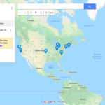
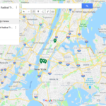
I had initially planned to have my network analysis praxis build on the work I had started in my mapping praxis, which involved visualizing the avant-garde poets and presses represented in Craig Dworkin’s Eclipse, the free on-line archive focusing on digital facsimiles of the most radical small-press writing from the last quarter century. Having already mapped the location of presses that had published work in Eclipse’s “Black Radical Tradition” list, I thought that I might try to expand my dataset to include the names and addresses for those presses that had published works captured in other lists in the archive (e.g., periodicals, L=A=N=G=U=A=G=E poets). My working suspicion was that I would find through these mapping and networking visualizations unexpected connections among the disparate poets in Eclipse and (possibly, later) those featured in other similar archives like UbuWeb or PennSound, which could potential yield new comparative and historical readings of these limited-run works by important poets.
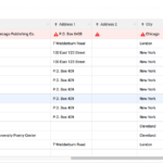
The dataset I wanted and needed didn’t already exist, though, and the manual labor involved in my creating it–I would have to open the facsimile for each of multiple dozens of titles and read through its front and back matter hunting for press names and affiliated addresses–was more than I was able to offer this week. So I’ve tabled the Eclipse work only momentarily in favor of experimenting with a more or less already-ready dataset whose network analysis I could actually see through from beginning (collection) to end (interpretation).
Unapologetically twee, I built a quick dataset of all the credited actors and voice actors in each of Wes Anderson’s first nine feature-length films: Bottle Rocket (1996), Rushmore (1998), The Royal Tenenbaums (2001), The Life Aquatic with Steve Zissou (2004), The Darjeeling Limited (2007), Fantastic Mr. Fox (2009), Moonrise Kingdom (2012), The Grand Budapest Hotel (2014), and Isle of Dogs (2018). As anyone who has seen any of Anderson’s films knows, his aesthetic is markedly distinct and immediately recognizable by its right angles, symmetrical frames, unified color palettes, and object-work/tableaux. He also relies on the flat affective delivery of lines from a core stable of actors, many of whom return again and again to the worlds that Anderson creates. Because of the way these actors both confirm and surprise expectations–of course Adrian Brody would be an Anderson guy, but Bruce Willis?–I wanted to use this network analysis praxis to visualize the stable in relation to itself and to start to pick at interpreting the various patterns or anomalies therein.
Fortunately IMDB automated a significant portion of the necessary prep work by providing the full cast list for each film and formatting each cast member’s first and last name in a long column–a useful tip I picked up while digging around Miriam Posner’s page of DH101 network analysis resources–so I was able to easily copy and paste all of my actor data into a Google Sheet and manually add the individual film data after. (I couldn’t copy and paste actor names from IMDB without grabbing character names as well, so I kept them, not knowing if they would end up being useful. For this brief experiment, they weren’t.)
-
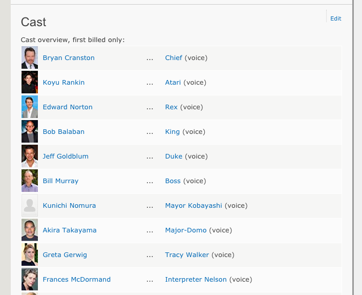
- Easily copied
-
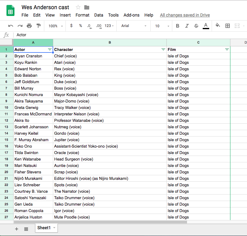
- Easily pasted
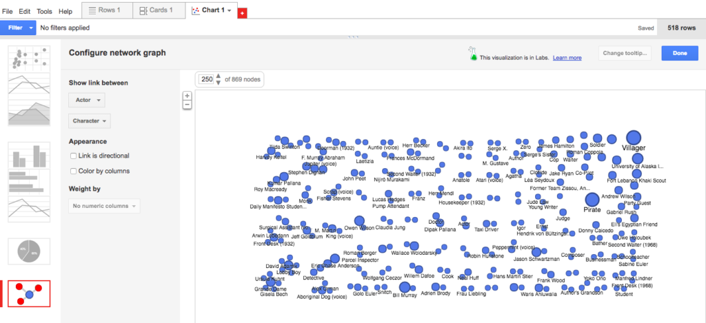
I used Google’s Fusion Tables and its accompanying instructions to build a Network Graph of the Anderson stable, the final result of which you can access here. As far as other tools went, Palladio timed out on my initial upload, buffering forever, and Gephi had an intimidating interface for what I intended to be a light-hearted jaunt. Fusion Tables was familiar enough and seemed to have sufficient default options for analyzing my relatively small dataset (500-ish rows in three columns), so I took the path of least resistance, for now.
A quick upload of my Sheet and a + Add Chart later, my first (default) visualization looked taxonomical and useless, showing links between actor and character that, as you might expect, mapped pretty much one-to-one except in those instances where multiple actors played generic background roles with identical character names (e.g., Pirate, Villager).
A poorly organized periodic table of characters
I changed the visualization to instead show a link between actor and film, and was surprised to find that this still didn’t show me anything expected (only one film?) or intriguing. Then I noticed that only 113 of the 449 nodes were showing, so I upped the number to show all 449 nodes. Suddenly, the visualization became not only more robust and legible, but also quite beautiful! Something like a flower bloom, or simultaneous and overlapping fireworks.
-
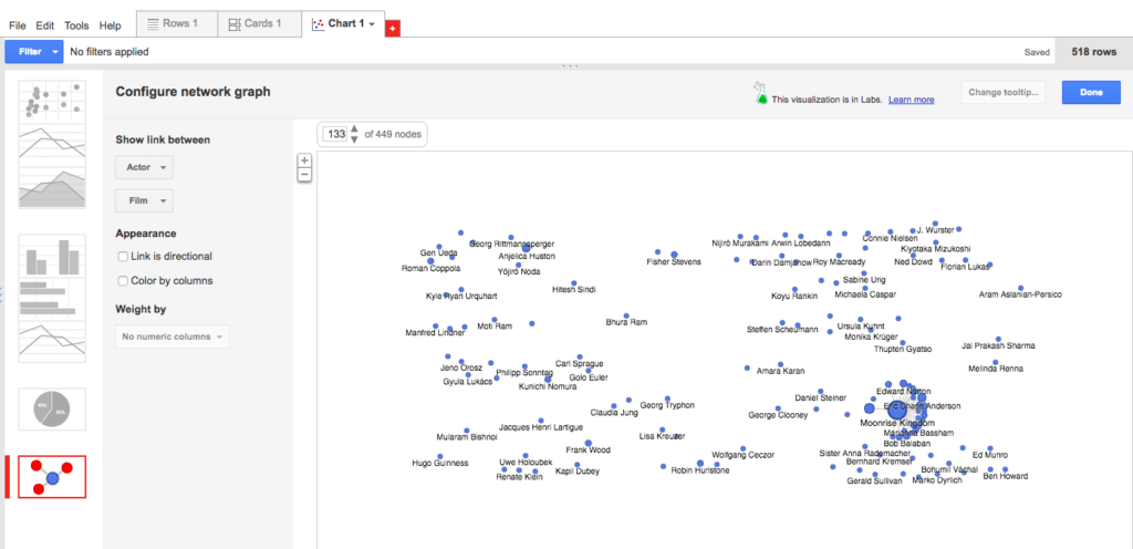
- Some nodes showing
-
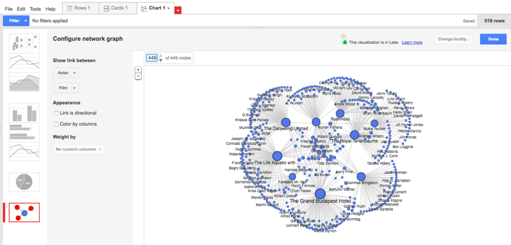
- All nodes showing
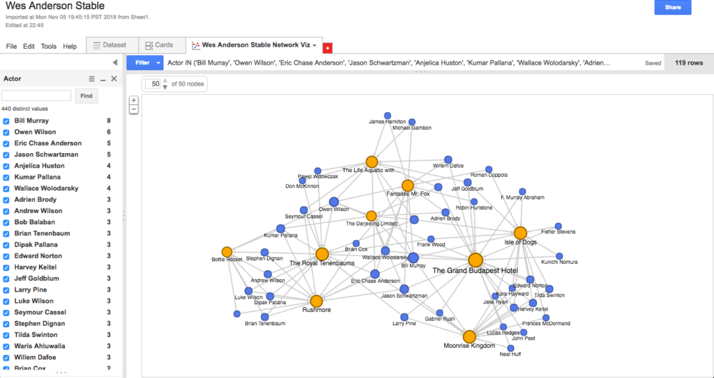
Beautiful as the fireworks were, I felt like the visualization was still telling me too much information, with each of the semi-circles consisting primarily of actors who had one-off relationships to these films. Because I wanted to know more about the stable of actors and not the one-offs, I filtered my actor column to include only those who had appeared in more than one of Anderson’s films (i.e., names that showed up on the list two or more times). I also clicked a helpful button that automatically color-coded columns so that the films appeared in orange and the actors in blue. This resulted in a visualization just complex enough to be worth my interrogating and/or playing with, yet fixed or structured enough to keep my queries contained.
-
- Network of repeat offenders
As far as reading these visualizations go, it’s something like this: Anderson’s first three films fall bottom-left; his next three films fall top-center; and his three most recent films fall bottom-right. Thus, the blue dots bottom-left are actors featured among the first three films only; blue dots bottom-center are actors who appear consistently throughout Anderson’s work; and blue dots bottom-right are actors included among his most recent films. As you can see by hovering over an individual actor node: the data suggests (e.g.) that Bill Murray is the most central (or at least, most frequently recurring) actor in the Anderson oeuvre, appearing in eight of the nine feature-length films; meanwhile, Tilda Swinton, along with fellow heavyweights Ed Norton and Harvey Keitel, appears to be a more recent Anderson favorite, surfacing in each of his last three films.
Also of interest: the name Eric Chase Anderson sits right next to Murray at the center of the network; Eric is the brother of Wes, the illustrator of much of what we associate with Wes Anderson’s aesthetic, and apparently also an actor in the vast majority of his brother’s films. (I’m not sure this find would have surfaced as quickly without the visualization.)
-
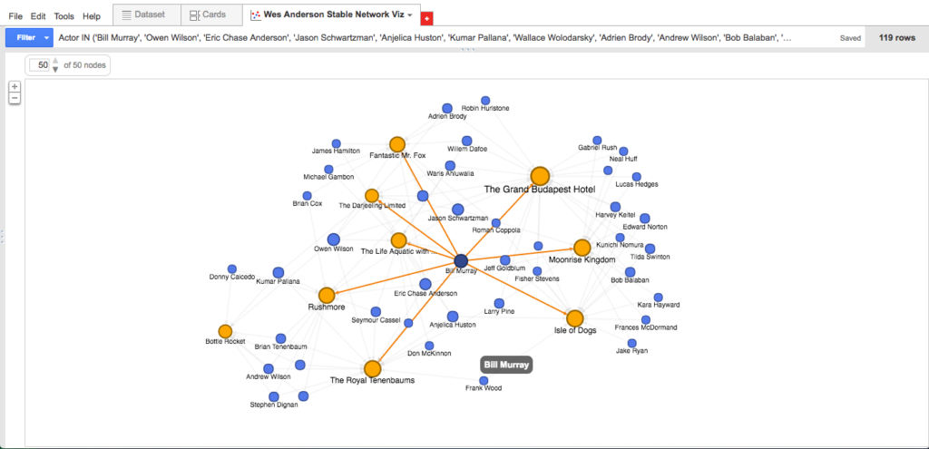
- Bill Murray in eight
-
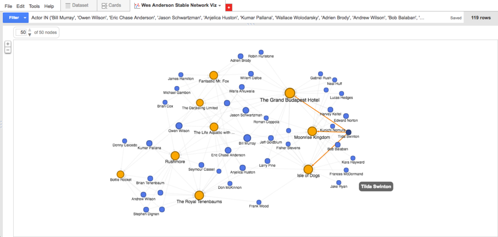
- Tilda Swinton in three
Elsewhere, the data suggests that Anderson’s first film Bottle Rocket was more of a boutique operation that consisted of a relatively small number of repeat actors (8), only two of which–Kumar Pallana and Owen Wilson–appeared in films beyond the first three. Anderson’s seventh film The Grand Budapest Hotel, released nearly twenty years later, expanded to include a considerable number of repeat actors (22: the highest total on the list), nine of whom were first “introduced” to the Anderson universe here and subsequently appeared in the next film or two.
-
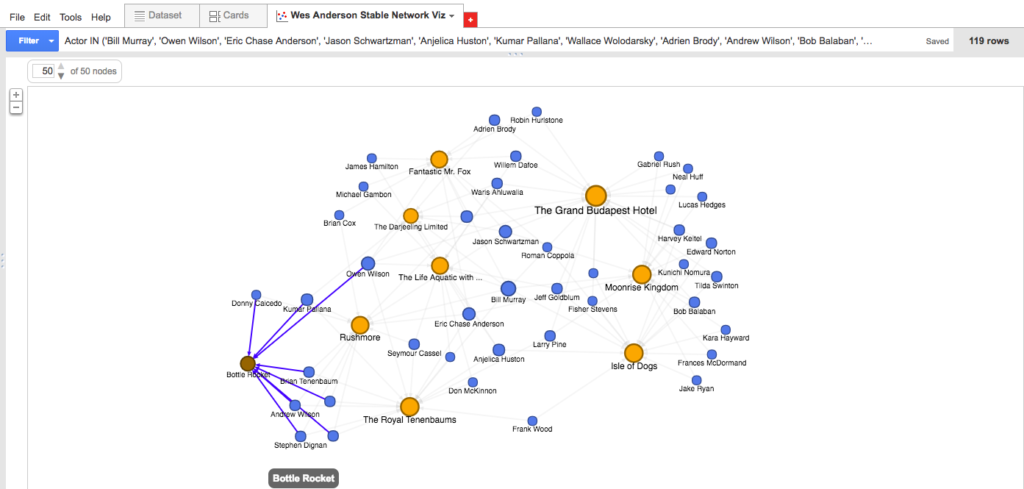
- Boutique Rocket
-
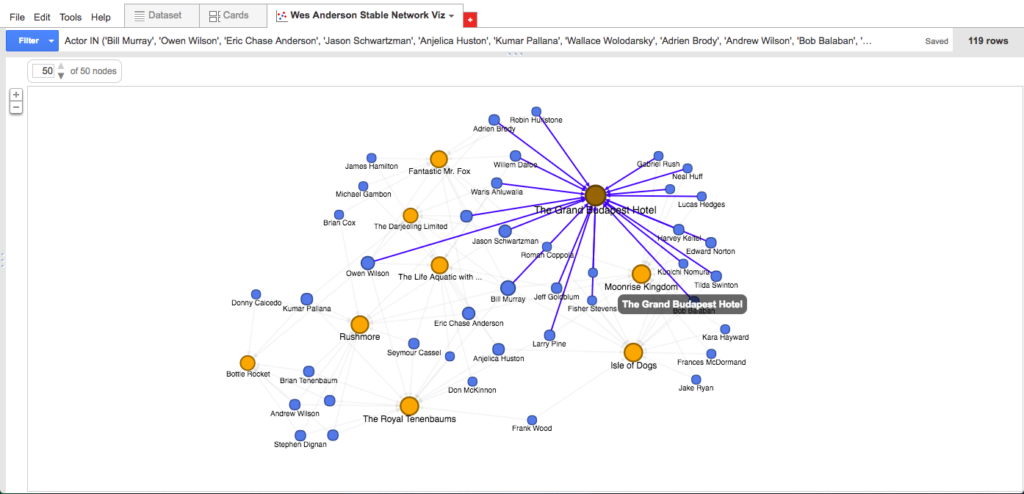
- Expand Budapest Hotel
I wonder what we would see if we visualized nodes according to some sort of sliding scale from “lead actor” to “ensemble actor” in each of these films, perhaps by implementing darker/more vibrant edges depending on screen time or number of lines? Would Bill Murray be more or less central than he is now? Would Eric Chase Anderson materialize at all?
And I wonder what opportunities there are to further visualize nodes based on actor prestige (say, award nominations and wins get you a bigger circle) or to create “famous actor” heat maps (maybe actors within X number of years of a major award nomination or win get hot reds and others cool blues) that might show us how Anderson’s casting choices change over time to include more big names. Conversely, what could these theoretical large but cool-temperature circles tell us about Anderson’s use of repeat “no-name” character actors to flesh out his wolds?
Further, I wonder if there are ways of using machine learning to analyze these networks and to predict the likelihood of certain actors’ being cast in Anderson’s next film based on previous appearances (i.e., the “once you’re in, you’re in” phenomenon) or recent success. Could we compare the Anderson stable versus, say, the Sofia Coppola or Martin Scorsese stables, to learn about casting preferences or actor “types”?